


Explaining Probability and Statistics through A/B Testing

📚 Note:
This post is 3rd part of the “Statistics Learning Series” — a set of concise, practical explainers designed to help you build strong foundations in Statistics for Business Management, Reporting and AI. Subscribe and go over these series only if you are planning to indulge in understanding Statistics more for your work!
This post brings together several core statistical concepts. If you'd like to dive deeper into any specific topic or have questions/clarifications, feel free to ping me on Substack — always happy to discuss.
Topics covered here include:
Inferential Statistics, Distribution Theory, Hypothesis Testing, and both Parametric & Non-Parametric Tests.
I. Introduction
Every product decision is a bet, you accept or not! You may not place chips on a table, but you’re still betting — on a product, feature, design, a phrase, a color, a layout. Sometimes it’s an instinct. Other times, it's a “best practice.” But beneath every confident launch is a lingering question: Did this really make a difference?
To keep this topic simple as its a tutorial, I am not discussing complex political, economical, behaviorial or business decisions to which this is very much applicable and makes more more impact but take a simple example like placing a button in a website. Lets Start!
Scenario: A product manager might swap a blue button for red. A marketer might revise a headline to be punchier. A designer might streamline the checkout flow to reduce friction. And as users begin to interact, a narrative forms: “B performed better than A.” But how can we know if that’s true — not just this time, but in general?
This is where probability and statistics kicks in into the story. Not as cold instruments, but the only way available today to interpreters of uncertainty. Their job is not to declare truth, but to help us reason honestly in the presence of randomness. They don't eliminate doubt — they help us quantify it, and act with clarity.
And there’s no better arena to watch them in action than the A/B test — a simple experiment that reveals the deep structure of evidence.
The A/B test is the fulcrum on top of which we want to explain many aspects of inferential statistics and probability in just one blog post. Each of these topics discussed here are complex, needs hours of study to understand so depending on your prior knowledge this could reveal to you more easily otherwise, do spend time to know them more but my only warning is, do not act that you know which can work against the experiments you do and be a disaster!

II. What Is A/B Testing? (Before the Math)
At its core, A/B testing is a controlled experiment. You take two versions of something — a landing page, an email, a user interface — and you show each version to a different, randomly selected group of users. The original version is often called the control, and the new or modified version is called the treatment or variant.
(I Know the devil in you is kicking in saying I already know this, but I leave it to you to read more and decide :) )
Each group interacts with their assigned version, and you track how they behave. You might be measuring whether they click a button, how long they stay on the page, whether they make a purchase, or how much they spend. These outcomes are what we call metrics, and they’re the heartbeat of the test.
For example, suppose you're testing two headlines. Group A sees the original headline and 30% of them click. Group B sees the new headline and 36% click. On the surface, it looks like the new headline is better. But A/B testing doesn’t just ask which version has the higher number. It asks a deeper question: Is that difference real — or just a product of chance?
Because humans are unpredictable. No matter how large your sample, randomness creeps in. One group may have had more motivated users by luck. Another may have loaded during festival time. A/B testing forces you to wrestle with this randomness with the support of Statistics and determine whether the pattern you see is likely to repeat.
The entire process hinges on one critical assumption: that the only difference between the two groups is the version they received. Everything else — from user demographics to time of day — should be balanced by randomization. That’s what makes the comparison fair. And that’s what allows statistics to do its work. Statistics will fail miserably if your cannot guarantee the randomness.
III. The Role of Probability: Modelling the Randomness
When you run an A/B test, you’re stepping into a world filled with uncertainty. Every user who visits your site faces a choice: click or not click, stay or leave, convert or abandon. You might think of this as a personal decision — and it is — but in the language of statistics, it’s also a random event. And randomness, for all its chaos, has a pattern.
Probability is how we describe that pattern. It’s the mathematics of chance — a way to talk about the likelihood of outcomes, even when we can’t predict any single case. It doesn’t tell you what will happen, but it gives you a structured expectation of what’s likely to happen over time.
If you flip a fair coin, the probability of heads is 0.5. But flip it 10 times, and you might get 4 heads. Or 7. That’s variation. Flip it 1,000 times, and you’ll probably land close to 500 heads. That’s convergence — and it's what makes probability useful. It allows us to understand randomness not as noise, but as something measurable.
In A/B testing, each user’s action can be thought of like a weighted coin toss. Maybe they have a 30% chance of clicking the button. You don’t know the exact probability, but if you watch enough users, their behavior begins to reveal it. That’s your window into the truth.
But here's the catch: you rarely get to observe everyone. You test a sample — a small slice of the full population. And when you do, randomness becomes your companion again. Even if two versions are identical in the population, your sample might show a difference — just by chance.
This is why probability is foundational to statistics. It sets the stage. It helps you model what could happen, so you can judge whether what did happen is surprising — or expected.
IV. Sampling and the Nature of Variation
In an ideal world, you'd run your A/B test on every user who might ever interact with your product. That would eliminate randomness. It would give you the full truth.
But in reality, that’s impossible.
You only get to observe a sample — a finite number of users who happen to land on your site during the test window. This introduces a fundamental tension in statistics: we want to make claims about the population, but we only see a subset. And that subset will always carry noise.
Even if Version A and Version B are equally good in the full population, the group of 500 users who saw A and the 500 who saw B might behave differently — simply due to chance. One group might have more loyal users, another might hit a slower server response. These small differences, when magnified through conversion rates, can look like real effects.
This is where statistics becomes more than just math — it becomes a philosophy of uncertainty. We accept that we don’t have perfect knowledge. But by studying how samples behave, we can still draw reliable conclusions.
So, what do we actually observe in a sample? Usually, it’s one of two things:
A proportion, when the outcome is binary (clicked or didn’t click)
A mean, when the outcome is continuous (seconds on page, dollars spent)
Each tells us something different. But both are subject to sampling variation. That means we don’t just want to look at the raw number — we want to understand how much it might vary if we ran the test again. We cannot run these tests for ever and fight or confuse on the outcomes but rather have the confidence to explain the situation well so we can move ahead with the decision.
And that brings us to the concepts of sample proportions, sample means, and standard error — the tools we use to make sense of the noise.
V. Proportions and Means: The Two Faces of Measurement
Suppose you’re running an experiment to see whether changing a CTA increases click-throughs. This is a classic binary outcome: either the user clicks (1), or they don’t (0). You show Version A to 500 users and get 150 clicks. You show Version B to another 500 users and get 180 clicks. That gives you:

These are sample proportions — your best estimates of the underlying probability of a user clicking. You don’t know the true conversion rate in the full population, but this is what your sample tells you.
In another experiment, let’s say you’re comparing two checkout flows, and you want to measure how long users spend on the payment page. Now your outcome isn’t binary — it’s continuous. Each user spends a different amount of time: 27.3 seconds, 31.1 seconds, 33.0 seconds, and so on. You take the average of all these values to compute the sample mean.
Version A: average checkout time = 32.5 seconds
Version B: average = 27.8 seconds
Whether you’re measuring a proportion or a mean, the principle is the same: you're using your sample to estimate a value that exists in the broader population. But your estimate will vary from sample to sample. And we need a way to describe how much it might vary — that’s where the standard error comes in.
VI. The Sample Mean and the Standard Error: Trusting the Average
Imagine standing at a shoreline, tossing a stone into the waves. Each splash lands somewhere slightly different — not because you aimed poorly, but because the sea is always in motion. Sampling is like that. Every test you run is a stone thrown into the sea of randomness. The results will vary — but the average gives us a center to hold on to, to understand how, you need to learn the Central Limit Theorem, explained later in this post.
The sample mean, whether it's of page views, revenue, or time spent, is our estimate of the “true” average behavior of all users — the population mean. But because we’re working with a sample, not the full population, we must ask: how much trust can we place in this mean?
Enter the standard error. It tells us how much our sample mean (or proportion) would fluctuate if we repeated the test with different random users. The more variability in your data — and the smaller your sample — the higher the standard error. It’s a measure of uncertainty, a quiet reminder that no single test tells the full story.
For a sample mean, the standard error is calculated as:

Where:
s is the sample standard deviation (how spread out your data is)
n is your sample size
If you're comparing two means — say, checkout times from two versions — you’ll compute the standard error of the difference. The same holds for proportions.
This leads to a powerful idea: not all differences are meaningful. A small difference might be just random fluctuation — or it might be real. We need a way to judge that.
VII. Confidence Intervals: Thinking in Ranges, Not Absolutes
One of the most intuitive ways to interpret uncertain data is through a confidence interval.
Let’s say your sample mean checkout time for Version A is 32.5 seconds, and your 95% confidence interval is [31.7, 33.3]. This means that if you ran the experiment 100 times, about 95 of those intervals would contain the true average checkout time of all users. You don’t know which 95 — but this is the logic of the long run.
In other words, we’re not saying the “true value” lies in this specific interval with 95% probability (that would be Bayesian logic). We’re saying the process of creating this interval gives us reliable coverage over repeated samples.
If you’re comparing two versions:
And their confidence intervals do not overlap, that suggests a real difference.
If they do overlap, then the observed difference might just be noise.
Confidence intervals provide a fuller picture than a yes/no answer. They say: Here’s what we saw — and here’s how much uncertainty we have about it.
And behind all this — sample mean, standard error, confidence interval — lies a quiet force that makes it all possible: the Central Limit Theorem.
VIII. The Central Limit Theorem: Order Within Randomness
At first glance, randomness looks like chaos. Users behave unpredictably. Every sample you take gives you slightly different results. The world of experimentation appears messy, unstable — difficult to trust.
But the Central Limit Theorem (CLT) whispers a quiet reassurance: beneath the randomness, there is order.
The CLT tells us something remarkable. No matter what the underlying population looks like — whether user behavior follows a bell curve or not, whether clicks are rare or common — if you take enough samples, the distribution of their means will begin to resemble a normal distribution. That familiar bell-shaped curve.
Let’s break that down.
Suppose your users spend wildly different amounts of time on your site. Some leave immediately, some linger for minutes. The overall distribution is skewed, maybe with a long tail. But if you repeatedly take random samples of, say, 500 users, and you compute the average time for each sample, those averages will start to form a pattern. That pattern will look increasingly like a normal distribution — centered around the true population mean.
This happens regardless of the shape of the original data. That’s the magic. It’s as if the act of averaging filters out the chaos.
And it works for proportions, too. Each user either clicks or doesn’t — a binary outcome. But the proportion of clickers in large enough random samples will still follow a normal curve, thanks to the same logic.
Why does this matter?
Because most statistical tests — z-tests, t-tests, confidence intervals — assume that the differences in your sample statistics (means or proportions) are approximately normal. The CLT makes this assumption valid, even if the original data isn’t. It is the bridge between messy real-world behavior and clean, interpretable inference.
So when we compute a p-value or draw a confidence interval, we’re relying — quietly, confidently — on the Central Limit Theorem. It’s what allows us to make bold decisions from noisy data.
Now that we’ve built this foundation, we’re ready to walk through two real A/B testing scenarios:
One involving proportions — comparing click-through rates
One involving means — comparing average time spent
These will demonstrate how all the pieces — sampling, standard error, confidence intervals, CLT — come together into statistical tests, and how we use them to reason with real data.
IX. Scenario 1: Comparing Proportions — Did More People Click?
Let’s say you’re testing two versions of a landing page. The only difference is the call-to-action button text.
Version A says: “Start Now”
Version B says: “Get Started”
You randomly assign users to each version and track whether they click the button. After the test runs, you collect the following data:
Version A: 500 users, 150 clicks → 30% conversion rate
Version B: 500 users, 180 clicks → 36% conversion rate
At first glance, it looks like Version B wins. A 6% lift! But before celebrating, pause.
Could that 6% difference be just due to chance?
Could it have happened even if the two buttons are equally good?
To answer that, we perform a hypothesis test — a structured way to evaluate how surprising our result is under the assumption that there’s no real difference.
Formulating the Hypotheses
In a two-proportion test, we start with two competing ideas:
Null Hypothesis H0: There is no difference in click rates between A and B → pA=pB
Alternative Hypothesis H1: There is a difference → pA≠pB
Under the null, we assume both groups are drawn from the same population — so any observed difference is just sampling variation.
Step-by-Step: The Two-Proportion Z-Test
To test whether the observed 6% difference is statistically significant, we follow these steps:
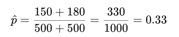
Calculate the pooled proportion:
Since we assume both groups are from the same population under H0, we pool their successes: You show Version A to 500 users and get 150 clicks. You show Version B to another 500 users and get 180 clicks. That gives you:
Calculate the standard error (SE) for the difference in proportions:
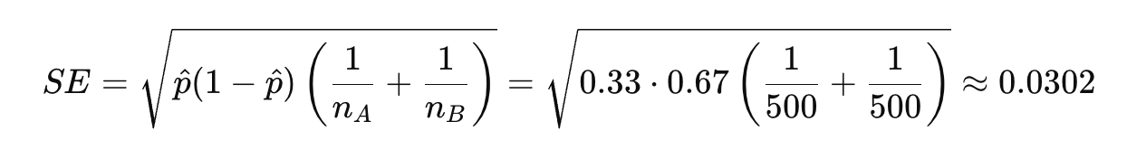
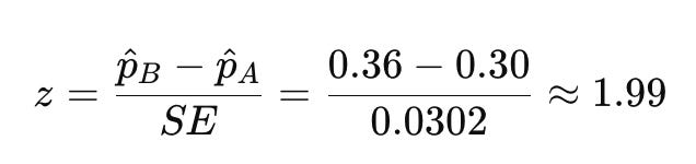
Compute the z-score:
This tells us how many standard errors the observed difference is away from 0 (the expected difference under the null):
Find the p-value:
A z-score of 1.99 corresponds (in a two-tailed test) to a p-value of around 0.046.

Interpreting the Result
A p-value of 0.046 means:
If there were no real difference between A and B, there’s about a 4.6% chance we’d see a difference this large or larger just due to random chance.
If we’re using a significance threshold of 0.05 (a common convention), then:
The result is statistically significant
We have some evidence that Version B performs better
But remember:
Statistical significance is not the same as practical significance. A 6% lift might be small or massive, depending on your product context. Also, this test doesn’t prove that B is better — it simply suggests that the observed difference is unlikely to be random.
X. Scenario 2: Comparing Means — Did People Stay Longer?
In this second test, you’re experimenting with two different checkout flows. One is your current version (let’s call it Version A), and the other is a redesigned experience (Version B) that aims to be simpler, faster, and less distracting.
Your goal? To reduce how long users spend in the checkout — not because time on page is bad, but because a long checkout often means confusion or friction.
After running the test on a large enough sample, you gather the following results:
Version A:
1000 users
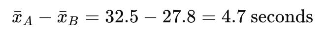
Average checkout time = 32.5 seconds
Sample standard deviation = 9.1 secondsVersion B:
1000 users
Average checkout time = 27.8 seconds
Sample standard deviation = 8.7 seconds
At first glance, it seems the redesign shaved off nearly 5 seconds. But again, we ask the now-familiar question:
Could this difference have arisen by chance, even if both designs are equally effective?
This time, we’re not dealing with binary clicks, but with continuous time data, so we’ll use a different statistical tool — the two-sample t-test.
Formulating the Hypotheses
As with the proportion test, we begin with our hypotheses:
Null Hypothesis H0: The average checkout time is the same in both versions → μA=μB
Alternative Hypothesis H1: The checkout times differ → μA≠μB
Step-by-Step: The Two-Sample t-Test
Calculate the difference between the sample means:

Compute the standard error (SE) of the difference in means:
Since the sample sizes are equal and large (n = 1000 for both), we use:
Calculate the t-statistic:

Find the p-value:
A t-score of 11.81 is extremely large. With degrees of freedom ≈ 2000, this corresponds to a p-value far smaller than 0.001.


Interpreting the Result
With such a tiny p-value, we can confidently reject the null hypothesis. The probability that we would see a difference this large if the two versions had the same true average checkout time is effectively zero.
So we conclude:
The redesigned checkout significantly reduced the average time spent on the page.
This result is not just statistically significant — it’s also practically meaningful. Saving 5 seconds on a task that’s often repeated at scale (hundreds of thousands of checkouts) can lead to smoother user experiences and possibly increased conversion rates.
But even here, humility matters.
We’re not claiming the new design is universally better in all contexts, or that it’ll continue performing identically tomorrow. We’re saying this: Given the data we collected, and the tools of probability and statistics, the evidence strongly supports a real improvement.
XI. The P-Value: A Measure of Surprise, Not Proof
After every statistical test — whether comparing click rates or average checkout times — we arrive at a number: the p-value. It's small or large. We compare it to 0.05. Sometimes we say, “It’s significant.” Other times, we shrug, “It’s not.”
But what does it actually mean?
The p-value answers a specific question:
If there were no real difference between A and B, what’s the probability that we would see a difference this big — or bigger — just due to chance?
That’s it.
It’s not the probability that A and B are equal.
It’s not the chance that the test “worked” or “failed.”
It’s simply a way of measuring how surprising your result is, assuming the null hypothesis is true.
In our first scenario, the p-value was 0.046. That means that if the two buttons were actually the same, you’d still see a 6% difference — or more — around 4.6% of the time. That’s rare enough that we took notice.
In our second scenario, the p-value was less than 0.001. That’s not just surprising — it’s astounding. The kind of result that demands attention.
But always remember: a p-value doesn’t tell you how big the effect is, or how important it is in practice. It’s a signal of strength, not of value.
XII. What the Test Tells You — and What It Doesn’t
When you run an A/B test and reject the null hypothesis, you’re saying, “The difference we observed is unlikely to have happened by chance.” That’s valuable. That’s evidence.
But it’s not the same as saying:
“Version B will always perform better.”
“This change will work for every user.”
“This experiment can’t be wrong.”
There’s always uncertainty. There’s always noise. There’s always a chance — however small — that the test led you astray. That’s why good experimenters replicate. They rerun. They test again.
On the other hand, failing to reject the null doesn’t mean the change doesn’t work. It just means your test didn’t provide enough evidence. Maybe your sample was too small. Maybe the effect was too subtle. Maybe your metric wasn’t sensitive enough.
Statistics doesn’t give us certainties. It gives us clarity.
XIII. Conclusion: A Philosophy of Evidence
Behind every click, every bounce, every conversion lies a story. A story of users making choices, often unpredictable, always entangled in noise. A/B testing is our attempt to listen to that story — not with certainty, but with structure.
Probability lets us model the chaos.
Sampling lets us study the world without knowing all of it.
The sample mean and standard error give us a lens into what we’ve seen — and what we might expect.
Confidence intervals help us think in ranges, not absolutes.
The Central Limit Theorem makes all of this work.
And statistical tests help us ask the only question that truly matters:
“Is what we’re seeing likely to be real?”
But at the end of it all, statistics isn’t just a toolkit for optimization. It’s a practice of humility. A way of saying:
We don’t know for sure — but here’s what the evidence suggests.
And that’s not a limitation. That’s a kind of brilliance.
In a world too fast to fully observe, too fragmented to fully control — we learn to act not from certainty, but from confidence.
Confidence earned not by instinct, but by science.
Not by guessing, but by listening carefully to the data.
That’s what makes A/B testing beautiful.
Not the lift. Not the win. But the discipline to ask: how do we know?
And the wisdom to let probability guide the answer.